Heading Error in Aeromagnetic Surveys: What It Is, Why It Matters, and How to Correct It

What is heading error?

This is a simplified, practical overview of heading error and one straightforward way to correct it using scalar + vector data.

In aeromagnetic surveys, a magnetometer is flown on a drone, helicopter, or aircraft to record the scalar total field and map subtle anomalies from faults, mineralization, intrusions, or man-made ferrous targets. In reality, the sensor also “sees” magnetic fields from its immediate surroundings—motors, batteries, wiring currents, and structural metals on the platform. As the platform yaws, pitches, and rolls, those local fields project differently into the measurement, creating an orientation-dependent artifact in the scalar trace. That artifact is heading error.

Even in the absence of platform induced effects, heading error is not strictly zero. A small residual heading error—often on the order of a few nT—is produced internally within the sensor due to imperfections.

Why should you care?

Heading error can be large enough to distort or mask the geologic signal you’re trying to interpret. A routine maneuver—like a swing or rotation of a towed sensor—can inject changes into the scalar channel that overwhelm the small field changes expected over short distances, making real anomalies harder to identify and map reliably. For context, the Magpie spec lists around 3 nT uncompensated heading error. That could be plenty large compared to many anomalies you care about in low-altitude drone surveys.

A real-world example of heading error

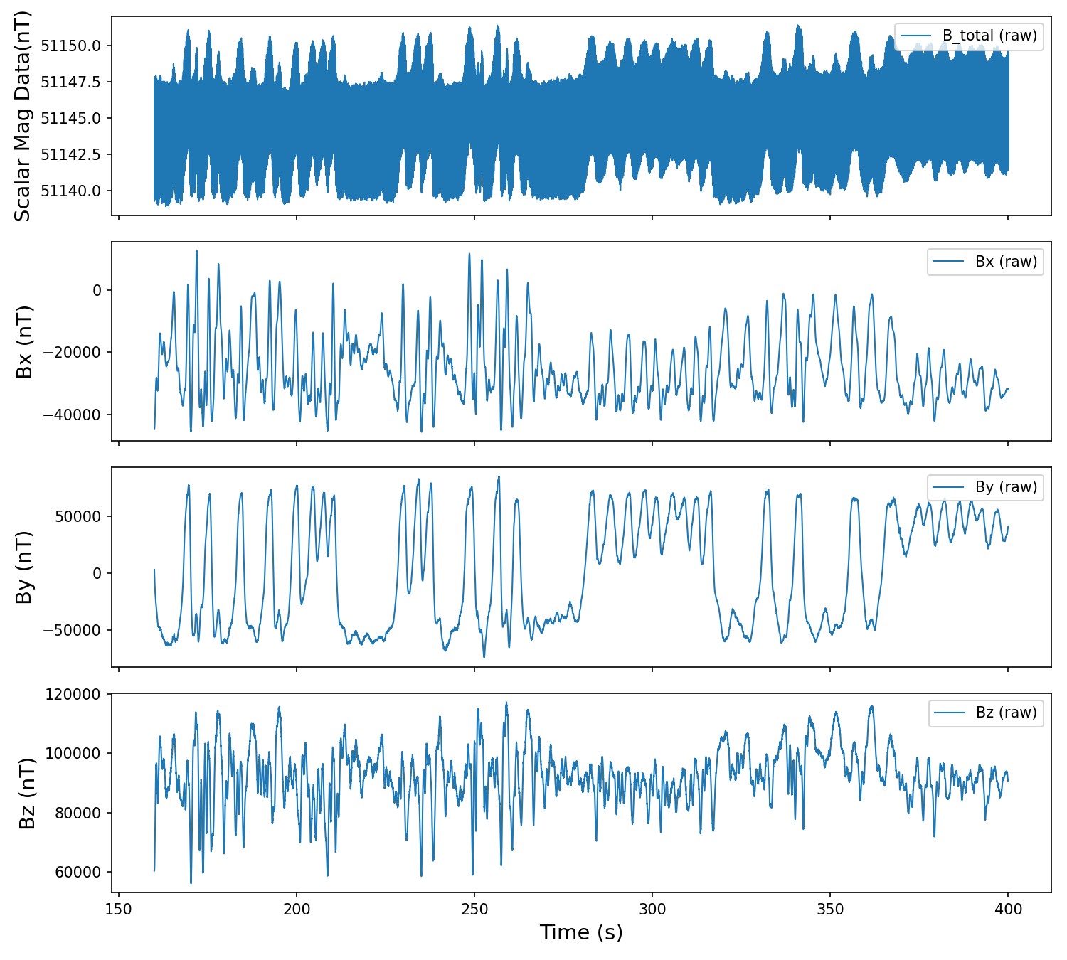
In one example recording, a Magpie is tethered beneath a drone. The drone ascends to ~30 ft and then stabilizes in roughly the same area, while the Magpie swings and rotates under the aircraft. As the package yaws, pitches, and rolls, the measured total field (centered near 51,144 nT) develops a clear quasi-periodic oscillation of about ~2 nT peak-to-peak with a period of a few seconds. That oscillation is the signature of heading error: the scalar measurement is being modulated by orientation-dependent magnetic contributions from the platform and nearby hardware (motors, wiring currents, structure, tether, etc.), not by a true change in the ambient Earth field.

The key clue is scale. Over the short distances involved in a swing (only a few feet of motion), the expected change in Earth’s field is typically well below 0.1 nT, so the dominant structure in this trace is an artifact rather than geology or natural gradients.

How to correct it Using QuSpin’s QTFM Vector Add-on

A scalar sensor alone can’t reliably separate true field variations from platform effects. QuSpin’s QTFM addresses this with an optional vector add-on that measures B_x(t), B_y(t), B_z(t) while the scalar channel records the total-field magnitude. With these vector components, you can build a simple, physically motivated model of the platform-induced contribution and remove it from the scalar trace.

A useful way to think about the measurement is:

• Measured scalar = (Earth field + geology) + (platform / payload magnetic contribution)

As the platform rotates, that platform/payload contribution can change in the sensor frame, even if the Earth field is essentially unchanged. The vector channels give you enough independent information to predict the orientation-dependent contamination and subtract it.

Note: This approach is general. If QTFM vector magnetometers are unavailable, you can use external vector magnetometers, provided they are rigidly mounted to the same reference frame as the QTFM sensor head so their components can be transformed consistently. You can also improve the correction model by including additional terms derived from other co-registered sensors in the same reference frame—for example linear and derivative terms from accelerometers and gyroscopes, or drive and commutation signals from onboard motor controllers and servos—to capture vibration, rotation-rate, and current-dependent magnetic signatures.

A simple model that works well in practice

A common starting point is to treat the “true” external field as approximately constant over a short calibration window, and model the heading-error contribution using a combination of:

• Linear terms in B_x, B_y, B_z
• Derivative terms dB_x/dt, dB_y/dt, dB_z/dt
• Quadratic and Cross terms like B_x², B_x*B_y, etc…

Linear terms often capture permanent/induced effects, while derivative terms are a convenient way to capture eddy-current-like or other dynamic coupling. Cross terms can help if you have slight axis non-orthogonality or subtle mixing between channels. The best model is use-case dependent—try a few variants and keep the simplest one that behaves well.

Worked example: heading error correction in Python

Below is a compact, workflow that matches the structure of the draft: load → (optional) filter → compute derivatives → least squares fit → subtract predicted artifact → save outputs. You can try this computation using the sample data set “Heading Error Correction Example Data Set.csv” provided by QuSpin and the python code snippets.

Step 1 — Load the data (scalar + vector)

Use the python snippet below to load the example data, or any dataset you wish to analyze. For this code to work, the data should be in the same directory as the python script. The code loads the example dataset from the CSV file and extracts the specific columns needed for heading-error correction: the time base, the scalar total-field measurement, and the three vector components. It converts the time column from milliseconds to seconds and shifts it so the first sample starts at t=0 seconds. Next, it converts each measurement channel into a NumPy array of floating-point values so the data can be processed efficiently with standard numerical routines. Finally, it estimates the sampling interval and sampling rate from the time stamps. That sampling-rate estimate is mainly a sanity check (to catch missing samples or irregular timing) and is also useful later if you apply frequency-domain filtering, since filter settings are specified in Hz.

import numpy as np
import pandas as pd
import matplotlib.pyplot as plt

LABEL_FONTSIZE = 14

fname = "Example Data Heading Error Correction.csv"
df = pd.read_csv(fname)

# --- Edit these column names to match your file ---
t_col = "Time (ms) [Main]"
scalar_col = "Mag Data[nT]"
x_col, y_col, z_col = "X", "Y", "Z"

# --- Extract arrays ---
t_ms = df[t_col].to_numpy()
t = (t_ms - t_ms[0]) / 1000.0  # seconds, starting at 0

B_total = df[scalar_col].to_numpy(dtype=float)
Bx = df[x_col].to_numpy(dtype=float)
By = df[y_col].to_numpy(dtype=float)
Bz = df[z_col].to_numpy(dtype=float)

# Sampling rate estimate (used for filtering)
dt = np.median(np.diff(t))
fs = 1.0 / dt
print(f"Estimated sampling rate: {fs:.2f} Hz")

# plot the raw data here
fig, axes = plt.subplots(4, 1, figsize=(10, 9), sharex=True)
axes[0].plot(t, B_total, label="B_total (raw)", linewidth=1.0)
axes[0].set_ylabel("Scalar Mag Data(nT)", fontsize=LABEL_FONTSIZE)
axes[0].legend(loc="upper right")

axes[1].plot(t, Bx, label="Bx (raw)", linewidth=1.0)
axes[1].set_ylabel("Bx (nT)", fontsize=LABEL_FONTSIZE)
axes[1].legend(loc="upper right")

axes[2].plot(t, By, label="By (raw)", linewidth=1.0)
axes[2].set_ylabel("By (nT)", fontsize=LABEL_FONTSIZE)
axes[2].legend(loc="upper right")

axes[3].plot(t, Bz, label="Bz (raw)", linewidth=1.0)
axes[3].set_ylabel("Bz (nT)", fontsize=LABEL_FONTSIZE)
axes[3].set_xlabel("Time (s)", fontsize=LABEL_FONTSIZE)
axes[3].legend(loc="upper right")
plt.tight_layout()
plt.savefig("Scalar_Vector_Raw.png", dpi=150)
plt.close()

When this code runs, it generates and saves the plot “Scalar_Vector_Raw.png”. Inspect this plot as a sanity check to make sure the plots look sensible. For the provided data set, you should observe a plot similar to this:

Step 2 – Filter Signals

Here we clean up the data before fitting the model. Two filters are especially useful:

1. Low-pass filter (important): removes high-frequency noise that can pollute derivatives and add jitter to the fit.
2. High-pass filter (optional): removes the slow baseline / DC level. If the absolute field value is less important than the changes caused by motion, consider removing it with a High-pass filter, which helps the fit focus on those changes instead of trying to “explain” the baseline.

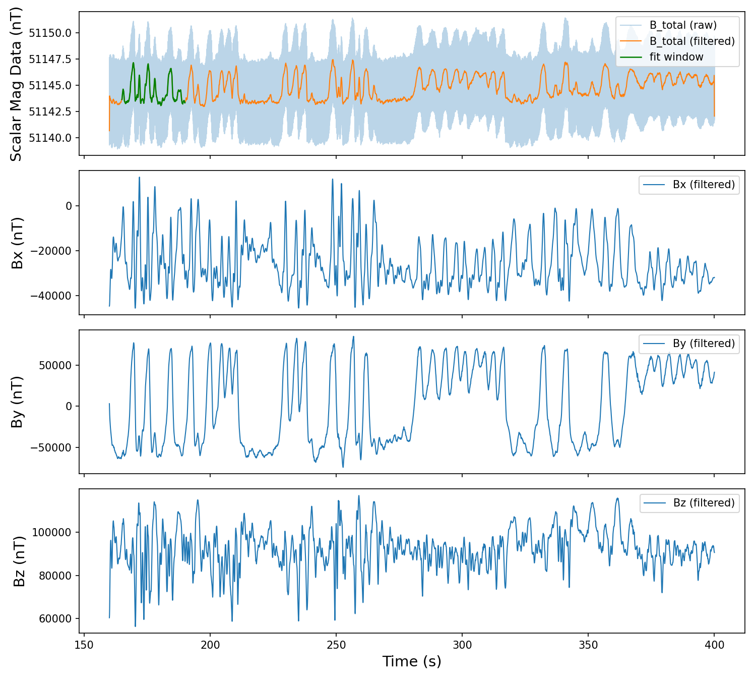
Optionally, you can also apply a notch to remove a narrow mains band (e.g., ~60 Hz) if it’s present. Below is a simple frequency-domain implementation that is easy to understand and works well for demonstration/tutorial code. Note that the code contains high-pass, low-pass, and notch filters, but we only apply a low-pass filter in the analysis. You should also specify a data segment the model will use to compute the coefficients. In this example, we segment the data from 90 to 145 seconds (green data in Figure 2).

def fft_highpass(x, fs, f_hp):
    """Remove frequencies below f_hp (Hz)."""
    x = np.asarray(x)
    X = np.fft.rfft(x)
    freqs = np.fft.rfftfreq(x.size, d=1/fs)
    X[freqs < f_hp] = 0
    return np.fft.irfft(X, n=x.size)

def fft_lowpass(x, fs, f_lp):
    """Remove frequencies above f_lp (Hz)."""
    x = np.asarray(x)
    X = np.fft.rfft(x)
    freqs = np.fft.rfftfreq(x.size, d=1/fs)
    X[freqs > f_lp] = 0
    return np.fft.irfft(X, n=x.size)

def fft_notch_band(x, fs, f_lo, f_hi):
    """Remove a narrow band of frequencies [f_lo, f_hi] (Hz)."""
    x = np.asarray(x)
    X = np.fft.rfft(x)
    freqs = np.fft.rfftfreq(x.size, d=1/fs)
    mask = (freqs >= f_lo) & (freqs <= f_hi)
    X[mask] = 0
    return np.fft.irfft(X, n=x.size)

# --- Toggle filters ---
use_lowpass = True    # optional: reduce high-f noise (helps derivatives)
use_highpass = False  # optional: remove baseline drift (focus on changes)
use_notch = False     # optional: remove mains band if present

# --- Filter settings (edit as needed) ---
f_hp = 0.05           # Hz
f_lp = 5.0            # Hz
notch_lo, notch_hi = 57.0, 64.0  # Hz (if needed)

# --- Fit window (seconds) ---
fit_start = 165
fit_end = 190

# Start from raw channels
B_total_f, Bx_f, By_f, Bz_f = B_total.copy(), Bx.copy(), By.copy(), Bz.copy()

if use_notch:
    B_total_f = fft_notch_band(B_total_f, fs, notch_lo, notch_hi)
    Bx_f = fft_notch_band(Bx_f, fs, notch_lo, notch_hi)
    By_f = fft_notch_band(By_f, fs, notch_lo, notch_hi)
    Bz_f = fft_notch_band(Bz_f, fs, notch_lo, notch_hi)

if use_highpass:
    B_total_f = fft_highpass(B_total_f, fs, f_hp)
    Bx_f = fft_highpass(Bx_f, fs, f_hp)
    By_f = fft_highpass(By_f, fs, f_hp)
    Bz_f = fft_highpass(Bz_f, fs, f_hp)

if use_lowpass:
    B_total_f = fft_lowpass(B_total_f, fs, f_lp)
    Bx_f = fft_lowpass(Bx_f, fs, f_lp)
    By_f = fft_lowpass(By_f, fs, f_lp)
    Bz_f = fft_lowpass(Bz_f, fs, f_lp)

fit_mask = (t >= fit_start) & (t <= fit_end)
if np.count_nonzero(fit_mask) < 2:
    raise ValueError("Fit window has too few samples. Adjust fit_start/fit_end.")

#plot the filtered data here
fig, axes = plt.subplots(4, 1, figsize=(10, 9), sharex=True)
axes[0].plot(t, B_total, label="B_total (raw)", linewidth=1.0, alpha=0.3)
axes[0].plot(t, B_total_f, label="B_total (filtered)", linewidth=1.0)
axes[0].plot(
    t[fit_mask],
    B_total_f[fit_mask],
    label="fit window",
    color="green",
    linewidth=1.2,
)
axes[0].set_ylabel("Scalar Mag Data (nT)", fontsize=LABEL_FONTSIZE)
axes[0].legend(loc="upper right")

axes[1].plot(t, Bx_f, label="Bx (filtered)", linewidth=1.0)
axes[1].set_ylabel("Bx (nT)", fontsize=LABEL_FONTSIZE)
axes[1].legend(loc="upper right")

axes[2].plot(t, By_f, label="By (filtered)", linewidth=1.0)
axes[2].set_ylabel("By (nT)", fontsize=LABEL_FONTSIZE)
axes[2].legend(loc="upper right")

axes[3].plot(t, Bz_f, label="Bz (filtered)", linewidth=1.0)
axes[3].set_ylabel("Bz (nT)", fontsize=LABEL_FONTSIZE)
axes[3].set_xlabel("Time (s)", fontsize=LABEL_FONTSIZE)
axes[3].legend(loc="upper right")
plt.tight_layout()
plt.savefig("Scalar_Vector_Filtered data.png", dpi=150)
plt.close()

After running this code, a plot titled “Scalar_Vector_Filtered data.png” is produced. Open it and observe how filtering the data has removed the baseline and noise components from the raw data.

Step 3 – Compute derivative channels from the vector components

In this step, the code takes the filtered vector measurements and computes their time derivatives. The motivation is simple: some heading-related artifacts don’t depend only on where the field components are, but also on how quickly they are changing as the sensor swings. Rapid changes in orientation can produce dynamic effects—often discussed in terms of eddy-current-like coupling or other time-dependent magnetic behavior in the platform—that show up strongly when the system is moving. Derivative terms give the model a way to “pay attention” to those dynamics. Practically, this also helps the fit capture oscillations in the scalar channel that align with the motion, even when the instantaneous vector components alone don’t fully explain the timing or amplitude. The derivatives are computed using a numerical gradient with respect to time, which is a robust, easy-to-interpret approach for evenly sampled data.

dBx = np.gradient(Bx_f, t)
dBy = np.gradient(By_f, t)
dBz = np.gradient(Bz_f, t)

Step 4 – Build the model predictors

This code assembles the “ingredients” the model is allowed to use to explain the scalar signal. Here we start with the physically motivated core: linear terms, derivative terms, quadratic and cross terms. You can expand or shrink this later with other terms if your setup benefits from it.

This step is where we translate the “physics-inspired model” into something a computer can fit. The code packages the model terms into a single matrix X, where each column is one predictor time series and each row corresponds to a time sample. The scalar time series we want to explain becomes the target vector y. Once the data are in this form, the coefficient-fitting problem becomes a standard regression task: find the set of weights that best combines the columns of X to match y.

baseline = np.mean(B_total_f[fit_mask])

# Columns: [constant, Bx, By, Bz, dBx, dBy, dBz, Bx^2, By^2, Bz^2, Bx*By, Bx*Bz, By*Bz]
X = np.column_stack([
    np.ones_like(t) * baseline,# baseline term
    Bx_f, By_f, Bz_f, # linear terms
    dBx, dBy, dBz, # derivative terms
    Bx_f**2, By_f**2, Bz_f**2, # quadratice terms
    Bx_f * By_f, Bx_f * Bz_f, By_f * Bz_f, # cross terms
])

# Target: scalar channel (filtered)
y = B_total_f
y_fit = y[fit_mask]

Step 5 — Solve for the coefficients (least-squares fit)

In this step, the goal is to learn the model coefficients—the numbers that tell you how strongly each predictor (the linear vector terms and the derivative terms) contributes to the heading-related variation seen in the scalar channel. Conceptually, we’re asking: “If the scalar trace is being contaminated by a platform field that depends on orientation and motion, what combination of the predictors best explains what we’re seeing?” The least-squares solver answers that question by finding the coefficient vector θ that minimizes the overall mismatch between the measured scalar time series and the model’s prediction. Because the model is linear in the unknown coefficients, this optimization is fast and stable—even for large datasets—and it tends to behave well as long as the dataset contains enough orientation/motion diversity to “excite” the different terms. If the sensor barely rotates (or if the vector channels don’t vary much), the fit can become under-constrained and coefficients may be noisy; that’s one reason swinging/attitude variation in the data is so valuable.

X_fit = X[fit_mask]
theta, *_ = np.linalg.lstsq(X_fit, y_fit, rcond=None)
print("theta =", theta)
resid = y_fit - X_fit @ theta
rmse = float(np.sqrt(np.mean(resid ** 2)))
mae = float(np.mean(np.abs(resid)))
sse = float(np.sum(resid ** 2))
sst = float(np.sum((y_fit - np.mean(y_fit)) ** 2))
r2 = float(1.0 - sse / sst) if sst != 0.0 else float("nan")
print(f"Fit metrics: RMSE={rmse:.6g}, MAE={mae:.6g}, R2={r2:.6g}")

# Plot filtered raw signal vs fit (fit window only).
plt.figure(figsize=(10, 5))
plt.plot(t[fit_mask], y_fit, label="filtered raw", linewidth=1.0)
plt.plot(t[fit_mask], X_fit @ theta, label="fit", linewidth=1.0)
plt.xlabel("Time (s)", fontsize=LABEL_FONTSIZE)
plt.ylabel("Scalar Mag Data (nT)", fontsize=LABEL_FONTSIZE)
plt.legend(loc="upper right")
plt.tight_layout()
plt.savefig("Filtered and Fit Overlay.png", dpi=150)
plt.close()

The output from print statements in the above code show the following:

theta = [ 1.00002765e+00  8.43994584e-05  3.53815383e-05  1.02192153e-04
 -9.73968094e-08  6.69160295e-07  3.98225378e-07 -1.72832669e-09
 -3.71298480e-10 -1.01361315e-09 -3.11228373e-10 -5.32758233e-10
 -1.88169884e-10]
Fit metrics: RMSE=0.0919011, MAE=0.0743073, R2=0.988541

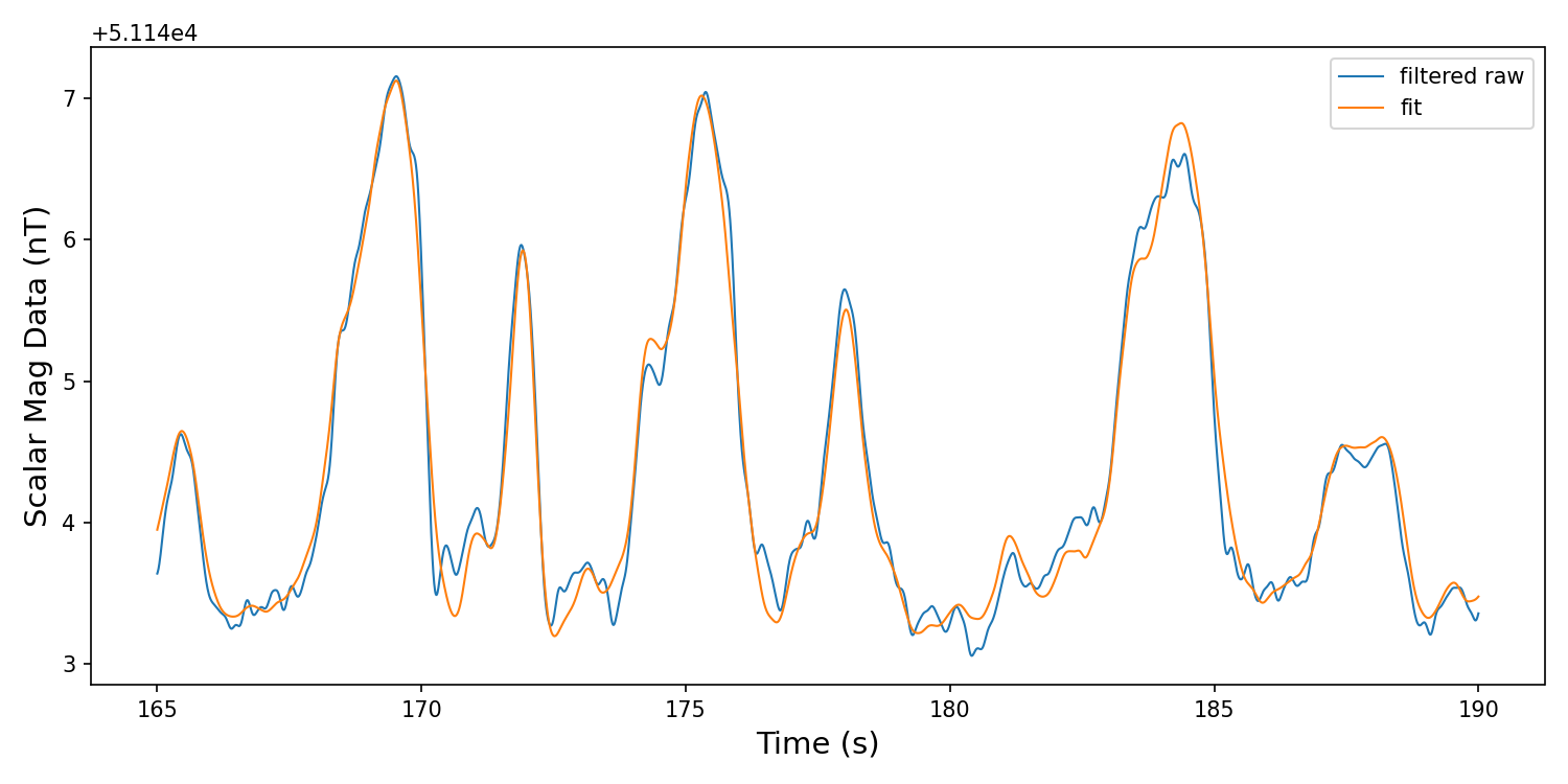
According to these results, the heading-error model fits the scalar data extremely well: the regression explains ~98% of the variance in the (filtered) scalar trace (R² = 0.986) with typical residual errors of only ~0.074 nT MAE and ~0.091 nT RMSE.

The code also generates an overlay plot (Filtered and Fit Overlay.png) that lets you visually assess the fit quality—shown here as Figure 3. You can see that the model captures the main swing-driven oscillations in the scalar trace quite well, though there are brief intervals where it under- or over-shoots the data, indicating some residual behavior that isn’t fully explained by the current set of model terms.

Step 6 — Predict the artifact and subtract it to form a compensated scalar trace

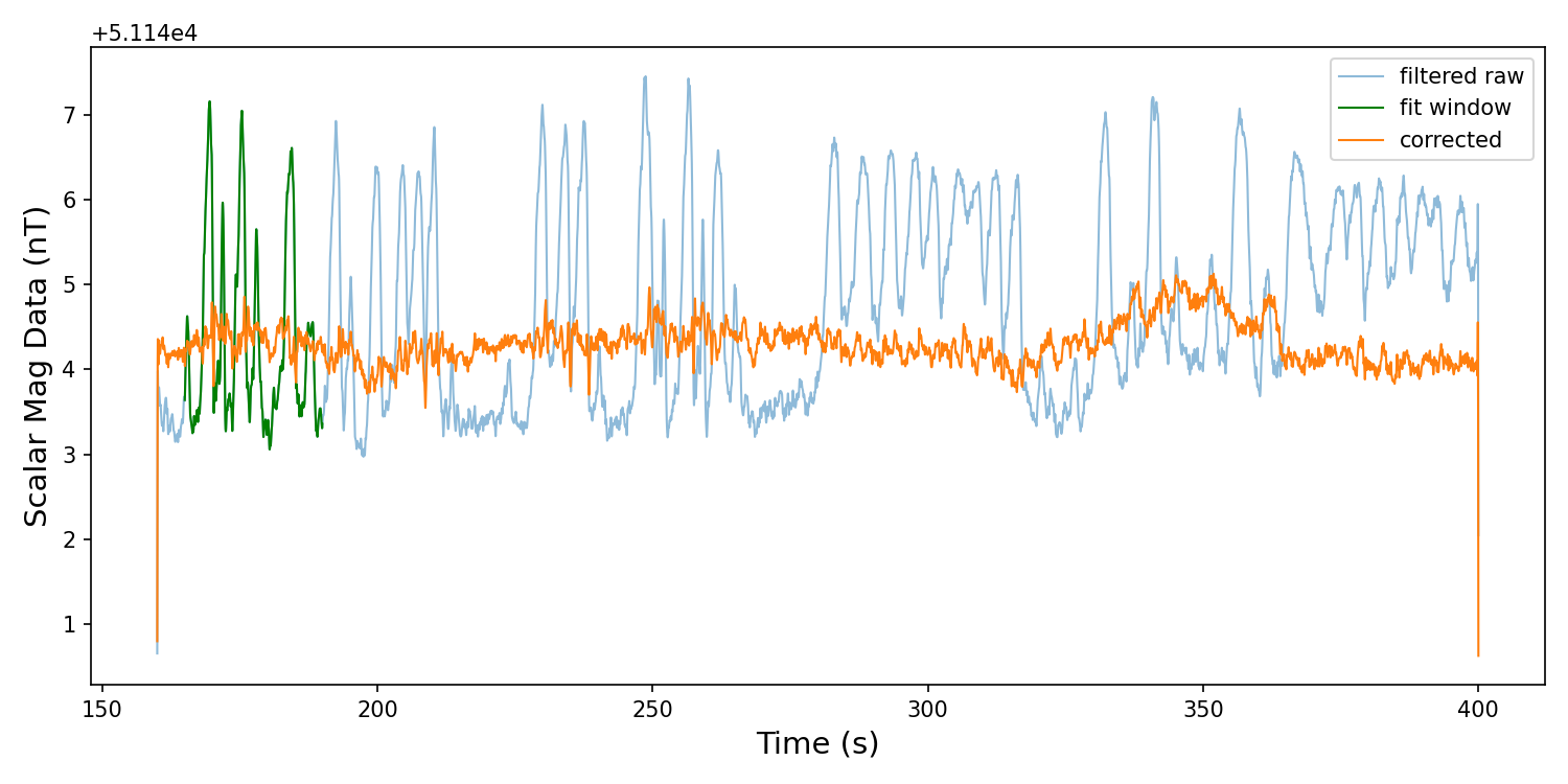
Once the coefficients are known, we use them to compute the model’s predicted scalar trace across the dataset. This predicted trace contains two conceptually different parts: a baseline (constant) contribution and a time-varying contribution driven by the vector channels and their derivatives. For heading-error correction, we care primarily about the time-varying part, because that’s what produces the oscillations correlated with swinging/rotation. The code therefore treats the time-varying part of the model as the artifact estimate and subtracts it from the measured scalar signal. The result is a compensated scalar trace where the heading-dependent oscillation is reduced, while the overall baseline is preserved—so you remove the “wobble” without artificially shifting the entire signal up or down. This is also the step where you’ll often see the most visually compelling before/after plots: the corrected signal should look markedly calmer during maneuvers, even though the raw data may have large oscillations

B_total_model = X @ theta

# Time-varying artifact estimate = model minus its constant baseline contribution
B_a_model = B_total_model - baseline

# Compensated scalar (baseline preserved)
B_comp = y - B_a_model

# Plot the filtered raw data and compensated data
plt.figure(figsize=(10, 5))
plt.plot(t, y, label="filtered raw", linewidth=1.0, alpha=0.3)
plt.plot(t[fit_mask], y[fit_mask], label="fit window", color="green", linewidth=1.0, alpha=0.3)
plt.plot(t, B_comp, label="corrected", linewidth=1.0)
plt.xlabel("Time (s)", fontsize=LABEL_FONTSIZE)
plt.ylabel("Scalar Mag Data (nT)", fontsize=LABEL_FONTSIZE)
plt.legend(loc="upper right")
plt.tight_layout()
plt.savefig("Filtered and Corrected Data Overlay.png", dpi=150)
plt.close()

The code generates a comparison plot (Filtered and Corrected Data Overlay.png) that you can use to visualize the results, which is shown in Figure 4. After applying the vector-based correction model, the orange trace stays much closer to a stable baseline, indicating that most of the heading-dependent artifact has been removed. The remaining small fluctuations in the corrected signal represent residual noise and any magnetic effects not captured by the current set of model terms.

Step 7 — Save outputs

This step writes the key time series to disk so you can generate publication-quality plots and compare results across model variants. Saving the artifact estimate is especially helpful because it lets you show (and verify) exactly what the algorithm believes is “heading error.”

out = pd.DataFrame({
    "t_sec": t,
    "B_total_filtered": y,
    "B_total_comp": B_comp,
    "B_a_model": B_a_model
})
out.to_csv("heading_error_compensated_timeseries.csv", index=False)
print("Wrote: heading_error_compensated_timeseries.csv"

For More Information

If you’d like a more technical treatment of aeromagnetic compensation, a good starting point is Derivation and Extensions of the Tolles–Lawson Model for Aeromagnetic Compensation, which presents a modern derivation and set of extensions to the classic Tolles–Lawson framework. It explains why specific model terms appear, how calibration maneuvers are designed, and how choices like filtering and model selection affect real-world performance. The references in that paper are also an excellent guide to the foundational Tolles–Lawson literature and other widely used compensation approaches.

For QTFM-specific guidance—especially around recommended maneuvers, sensor configurations and best practices—or if you’d like customized scripts tailored to your platform and mounting configuration, contact Jeff Orton at jorton@quspin.com