
In this walkthrough, we’ll take a QuSpin Neuro-1 optically pumped magnetometer recording from acquisition to source-level analysis. Along the way, we’ll cover signal cleanup, HALO-based sensor localization, subject coregistration, auditory evoked response analysis, and source localization using a linearly constrained minimum variance beamformer.
Introduction
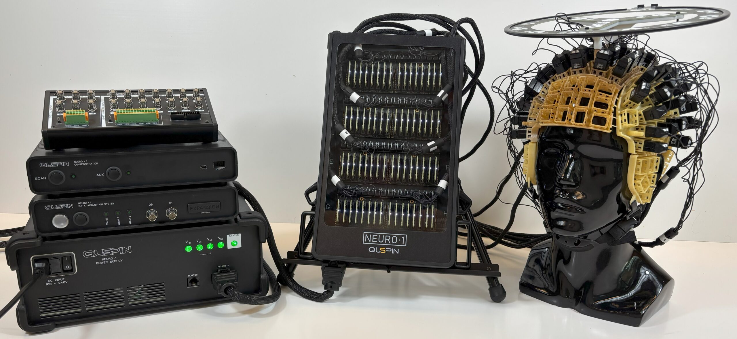
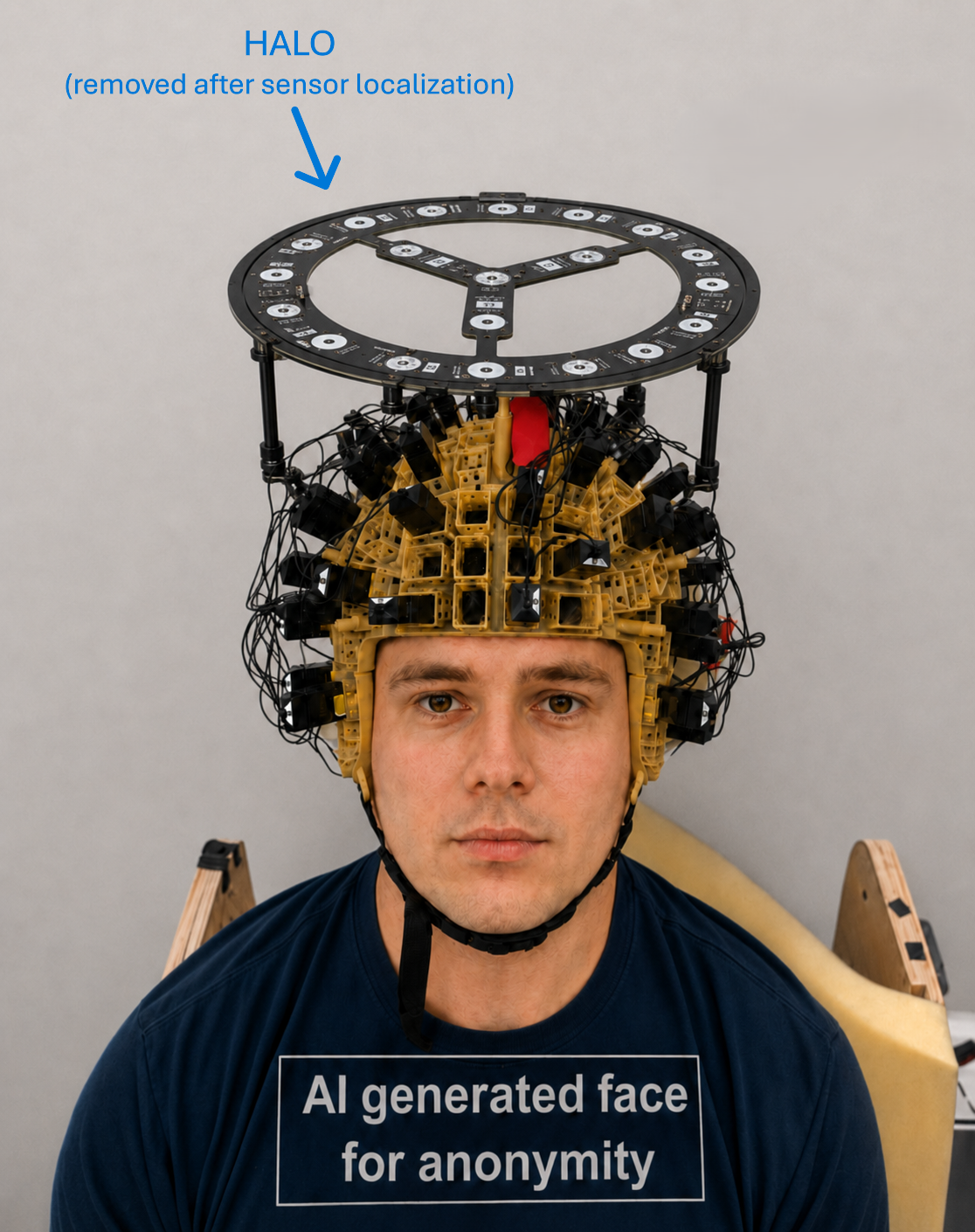
The Neuro-1 is QuSpin’s integrated OPM-MEG platform, combining QZFM Gen-3 triaxial sensors, miniaturized control electronics, a data acquisition system (DAQ), and a low-noise power supply into a single unified system. The N1 DAQ acquires data from 128+ sensors (up to 384 channels) with synchronous external analog and digital I/O, enabling precise stimulus timing. An API supports integration with LabVIEW, MATLAB, and Python. Sensor electronics have been miniaturized to SD-card size — compact enough to fit in a small backpack worn by the subject. The architecture is highly scalable and upgrade-friendly, with user-selectable single, dual, or triaxial sensing modes and built-in triaxial closed-loop operation.
This tutorial walks through a complete Neuro-1 OPM-MEG workflow: data collection, sensor localization, subject coregistration with FrameAlign, signal cleanup with homogeneous-field correction (HFC), and source localization with a landmark-guided LCMV beamformer. An auditory evoked response (AER) is used as the example paradigm. Each step is documented with the QuSpin tool or script used to produce the results shown.
The recording in this tutorial uses 192 channels from 64 triaxial QZFM Gen-3 zero-field OPMs, recorded inside a two-layer magnetically shielded room (Magnetic Shields Limited). Sensors are mounted in a semi-rigid helmet with 150 OPM slots for whole-head coverage.
Images of subjects in this tutorial have been altered using AI-generated faces to protect participant anonymity.
A Note about Coordinate Frames
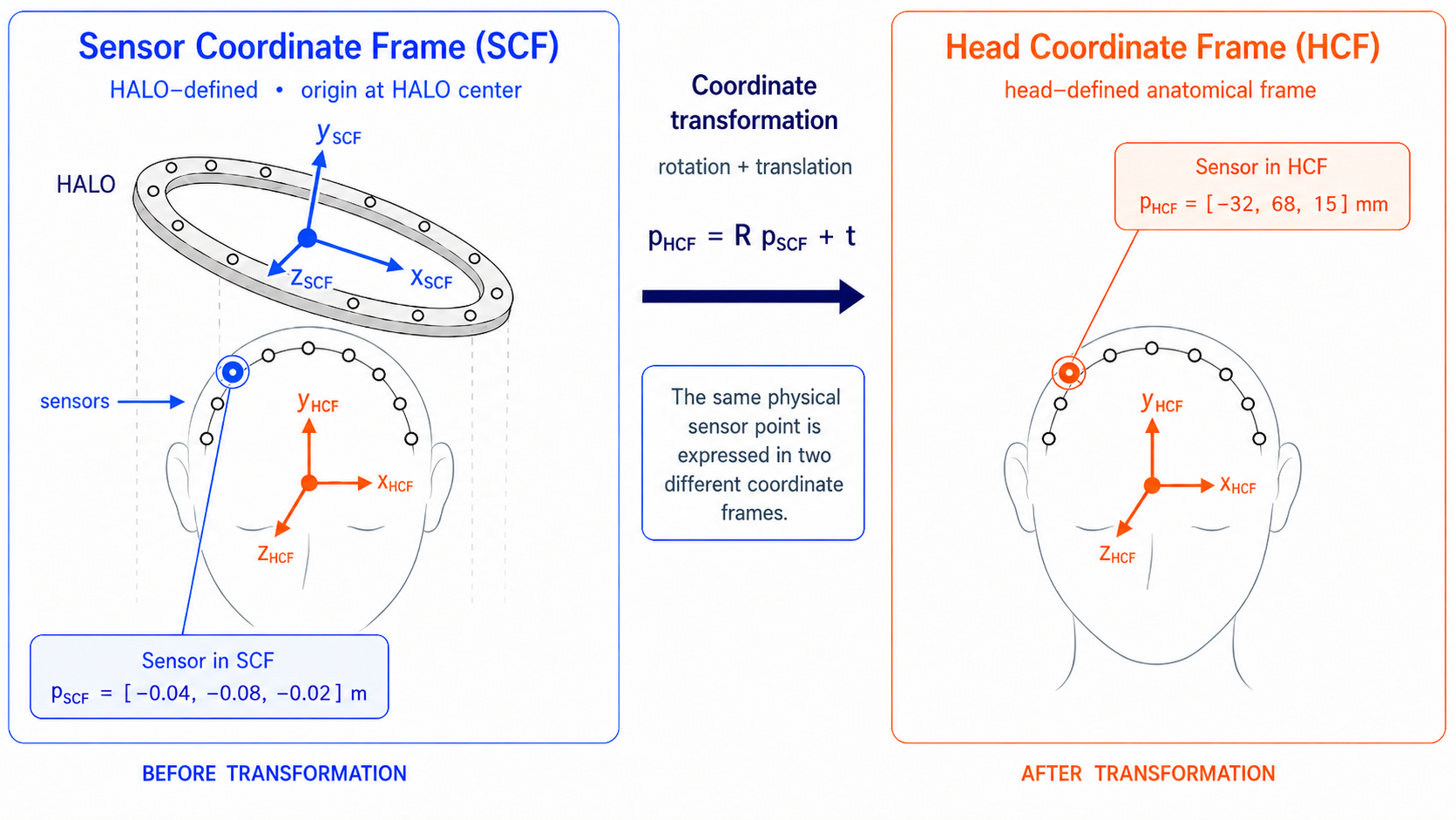
SCF — Sensor Coordinate Frame (meters)
Defined by the HALO system. When the HALO PCB coils activate, the OPM sensors measure the resulting magnetic fields and the software triangulates each sensor's position and sensitive-axis orientation relative to the PCB. All HALO outputs — sensor positions, orientations, and calibration gains — are expressed in SCF. SCF is used throughout signal processing, including HFC and beamforming. Internal files may label SCF as SCB; the data are identical.
HCF — Head Coordinate Frame (millimeters)
Defined by the subject's 3D face scan (or MRI/CT). Anatomically anchored to the subject, with the origin typically between the ear canals. Source locations and all visualization outputs are reported in HCF.
FrameAlign registers SCF to HCF by matching corresponding landmark points measured in both frames. The operator touches anatomical landmarks — nose tip, nasion, points near the ear canals, eye corners — with the HALO Pen while the OPM sensors record, placing those landmarks in SCF. The same landmarks are then identified on the subject’s 3D scan in HCF. FrameAlign pairs the corresponding points and solves for a 4×4 similarity transform: rotation, translation, and a scale factor that accounts for the meter-to-millimeter unit difference between the two frames. Applying this transform maps all HALO-localized sensor positions and orientations from SCF into HCF, linking the sensor array to the subject’s anatomy.
QuSpin Software
Three QuSpin tools cover the full workflow from data collection to source localization.
Workflow Summary
The workflow has two linked parts: geometry processing and MEG signal processing. The geometry steps establish where the sensors and subject landmarks are, and the signal-processing steps use that geometry to clean the data, compute evoked responses, and estimate source-level virtual electrodes.
| Step | Main input | Main output | Coordinate frame | Key tool / command |
|---|---|---|---|---|
| Collect HALO co-registration recording | HALO PCB positioned on subject with sensors in place | Raw co-registration recording (~30 s) | Native recording file | N1 software |
| Collect auditory evoked recording | Stimulus-triggered OPM session | Raw recording with digital or analog triggers | Native recording file | N1 software |
| HALO sensor localization | Short HALO PCB co-registration recording | Sensor positions, orientations, gains, and sensor OBJ | SCF | quspin.exe localize |
| HALO Pen fiducials | Pen touch recordings on face landmarks | Fiducial point CSV, XYZ, and OBJ | SCF | quspin.exe fiducial |
| FrameAlign coregistration | Subject 3D scan plus HALO Pen fiducials | SCF-to-HCF transform and combined geometry | HCF | FrameAlign |
| HFC (homogeneous field correction) and evoked response | Coordinate-annotated auditory FIF | Raw-vs-HFC PSD and D0-triggered evoked average | SCF sensor geometry from FIF metadata | quspin.exe hfc or MNE Tools |
| LCMV beamforming | HFC-cleaned epochs, SCF sensors, landmark-guided search regions | Temporal sources, OBJ models, virtual electrodes, SNR | Computed in SCF, reported in HCF | MNE Tools |
Data Collection: HALO and Auditory Evoked Recordings
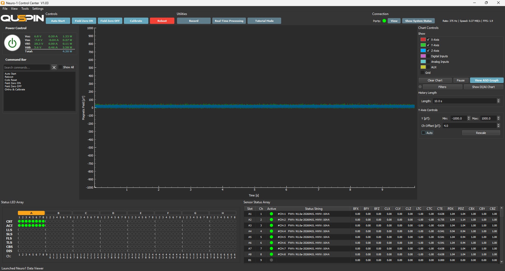
Download the N1 software and refer to the N1 user guide for installation and setup instructions. Then use the Neuro-1 software to configure your sensor channels, assign the auditory stimulus trigger to channel D0, and record the HALO and Audio Evoked stimulus data. When finished, the software saves either a .lvm or .fiff data file that is used in all subsequent processing steps.
Sensor Localization With HALO
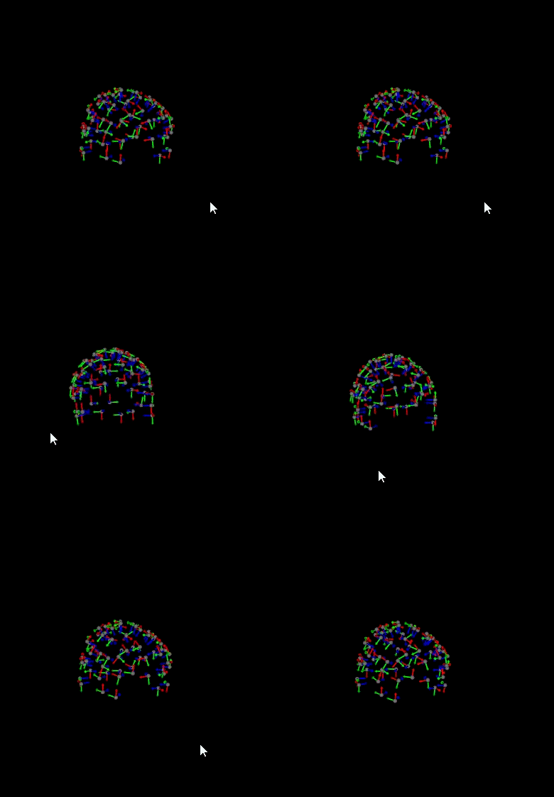
The HALO PCB is placed over the subject’s head during a sensor localization session. Its coils activate sequentially, and the OPM array response is used to compute each sensor’s position, orientation, and gain in the HALO-defined sensor coordinate frame (SCF). A co-registration recording takes roughly 30 seconds; typical accuracy is 1–2 mm position, 1–2° orientation, and ~1% gain. QuSpin AllTools or the quspin CLI outputs a CSV of results and an OBJ 3D model of the sensor configuration (Figure 5). After the sensor localization step, the HALO PCB is removed for the auditory evoked response recording and all subsequent steps.
Example Python Script
The script below calls quspin.exe localize on your HALO co-registration recording. Update the paths at the top and run from the folder containing quspin.exe.
import subprocess
from pathlib import Path

# ── Set your paths ────────────────────────────────────────────────
QUSPIN_EXE       = Path(r".\quspin.exe")
HALO_RECORDING   = Path(r"C:\your_data\halo_coreg_recording.lvm")
# ─────────────────────────────────────────────────────────────────

subprocess.run([
    str(QUSPIN_EXE), "localize",
    "--input-path", str(HALO_RECORDING),
    "--verbose",
], check=True)

# Outputs saved beside the recording:
#   <stem>_Localization_Results.csv  — positions, orientations, gains
#   <stem>_Sensor_3D_Model.obj/.mtl  — 3D model for visualization
print(f"Localization complete. Results saved alongside: {HALO_RECORDING}")
Subject Coregistration With the HALO Pen
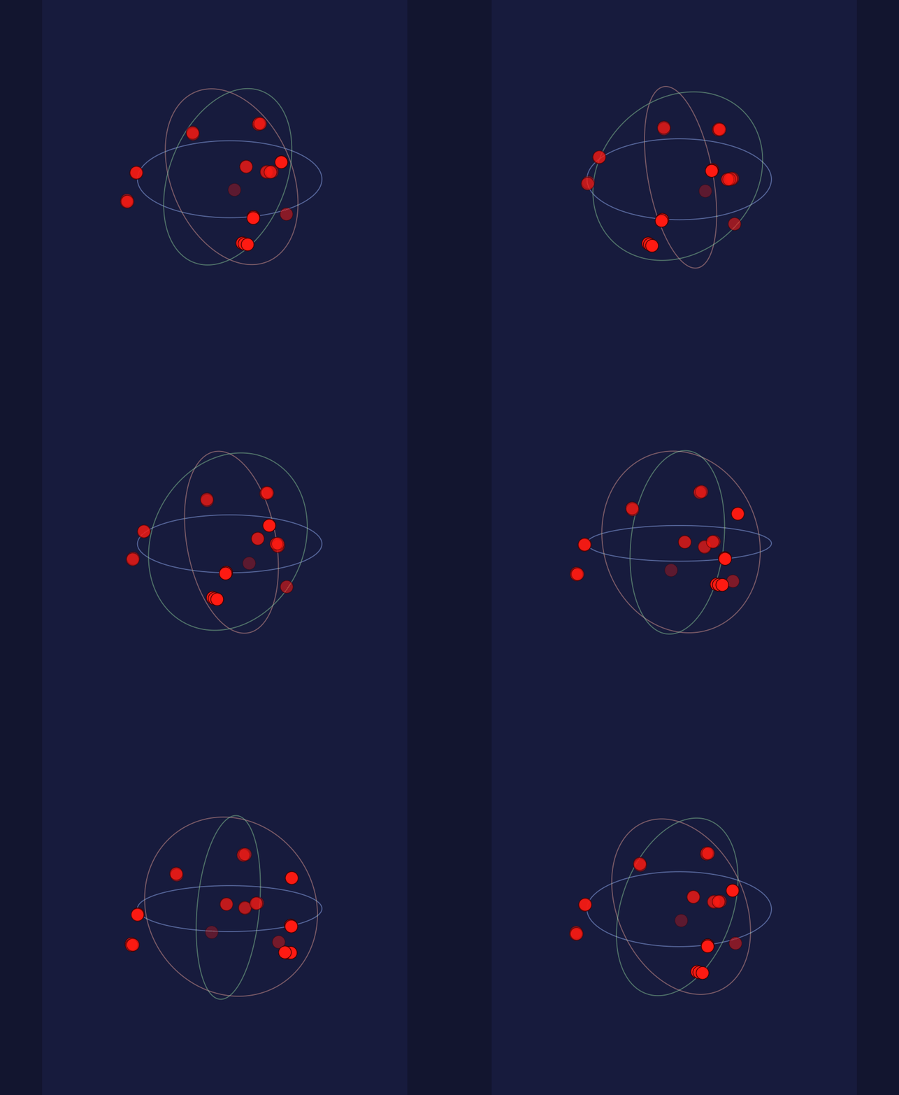
The HALO Pen is a handheld device with two orthogonal coils that activate at 29 Hz and 37 Hz when the operator presses the button. The OPM array measures those fields and projects the pen-tip position in SCF (Figure 6). Pen landmark acquisition takes roughly 30 seconds.
Touch the pen tip to recognizable anatomical landmarks that can also be identified on the subject’s 3D scan: nose tip, nasion, inner or outer eye corners, points near the ear canal or tragus, cheekbone points, and stable forehead locations. Well-spread landmarks constrain the transform globally and reduce sensitivity to any single point.
Example Python Script
The script below calls quspin.exe fiducial to localize your pen recording against a sensor localization CSV.
import subprocess
from pathlib import Path

# ── Set your paths ────────────────────────────────────────────────
QUSPIN_EXE       = Path(r".\quspin.exe")
LOCALIZATION_CSV = Path(r"C:\your_results\localization_results.csv")
PEN_RECORDING    = Path(r"C:\your_data\pen_recording.lvm")
# ─────────────────────────────────────────────────────────────────

subprocess.run([
    str(QUSPIN_EXE), "fiducial",
    "--localization-results", str(LOCALIZATION_CSV),
    "--measurement-path", str(PEN_RECORDING),
    "--verbose",
], check=True)

# Outputs saved beside the pen recording:
#   <stem>_fiducial_localization_results.csv — pen-tip positions in SCF
#   <stem>_fiducial_localization_results.obj — 3D point cloud for FrameAlign
print(f"Fiducial localization complete. Results saved alongside: {PEN_RECORDING}")
Frame Align: Mapping the Pen Points to the Head Coordinate Frame
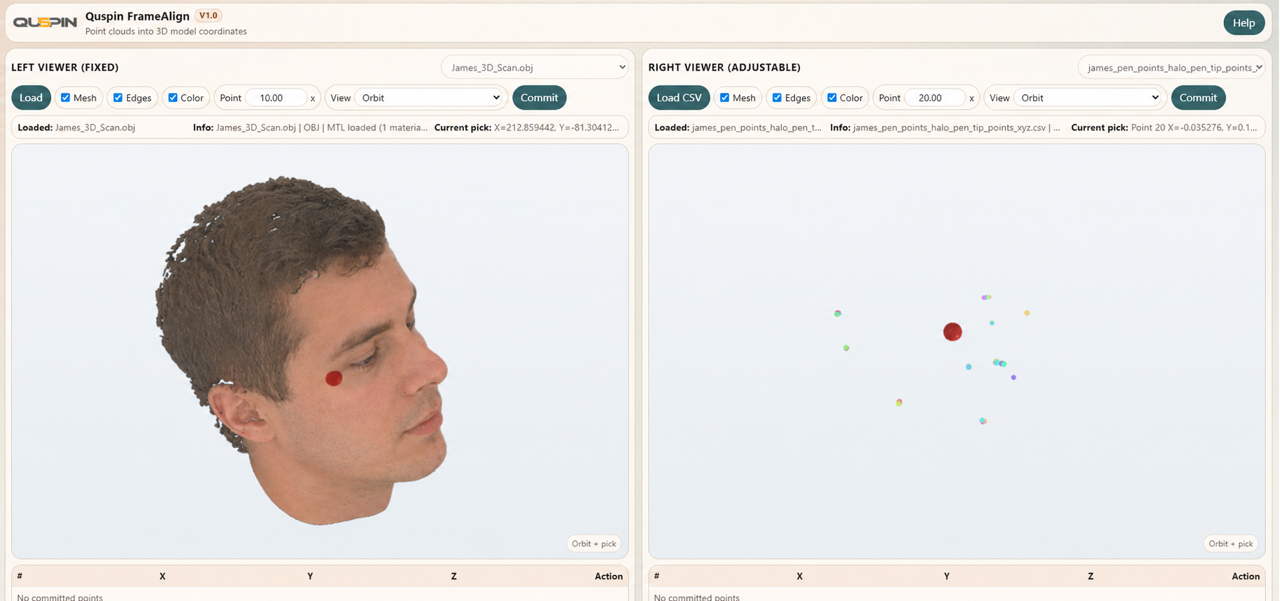
Open the subject’s 3D model in FrameAlign’s left viewer and the HALO Pen .xyz point cloud alongside it. The face point cloud used here was acquired with an Einscan H structured-light scanner. For each landmark, click the matching point on the 3D model and the corresponding pen point. The built-in solver computes a similarity transform — rotation, translation, and scale — that maps SCF pen points onto the HCF model (Figure 7).
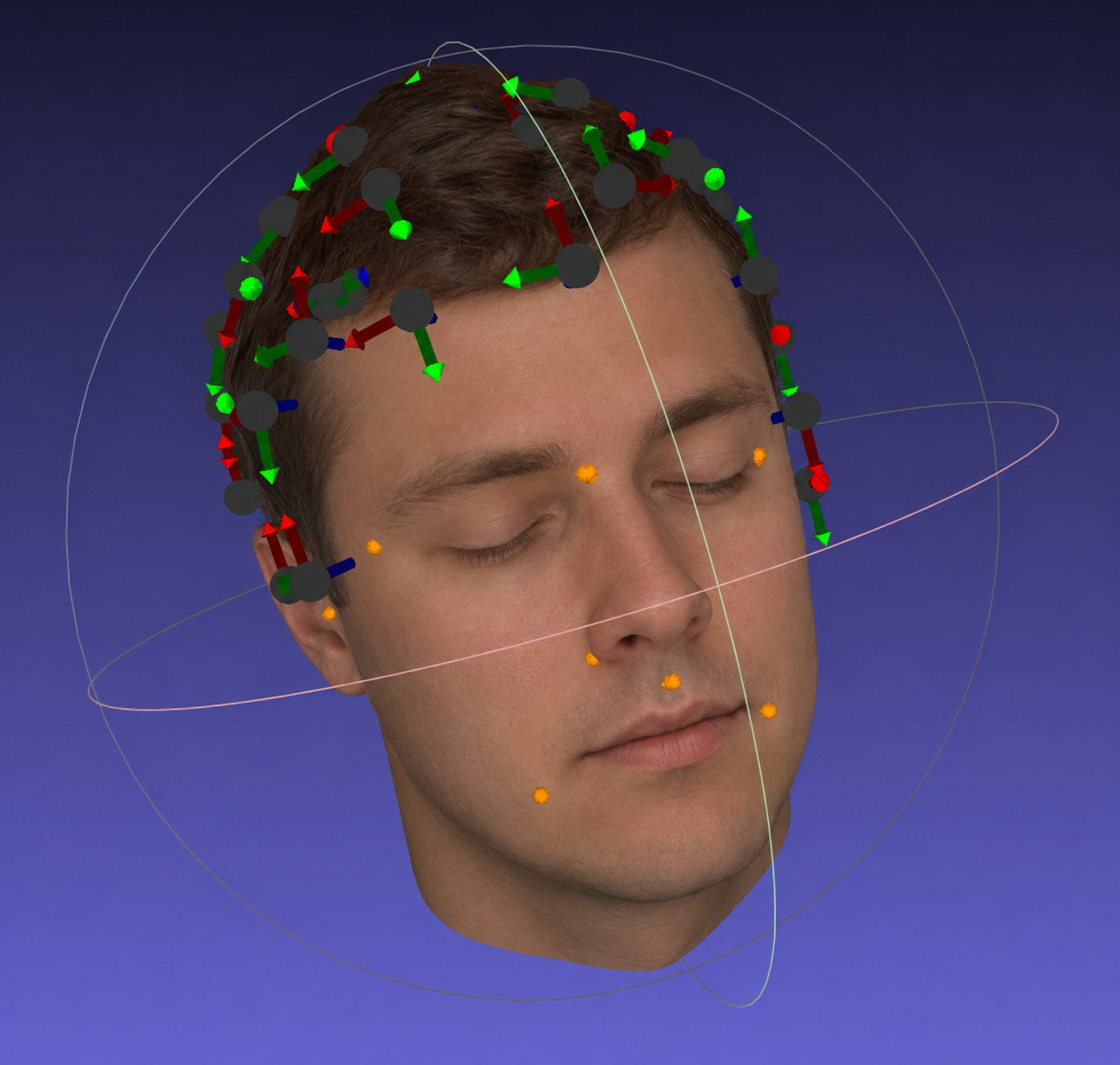
Once computed, apply this transform to map all HALO-localized sensor positions and orientations from SCF into HCF, linking sensor geometry to subject anatomy for source localization (Figure 8). Save the matrix below from your FrameAlign session.
Signal Cleanup With HFC
QuSpin AllTools writes the HALO-derived sensor coordinates and calibration gains into the .fif recording. Before proceeding, consider the full range of noise-suppression techniques available in the MNE platform — including higher-order signal-space separation (SSS), temporal SSS (tSSS), and reference-channel regression — and select the approach best suited to your experimental arrangement and data quality.
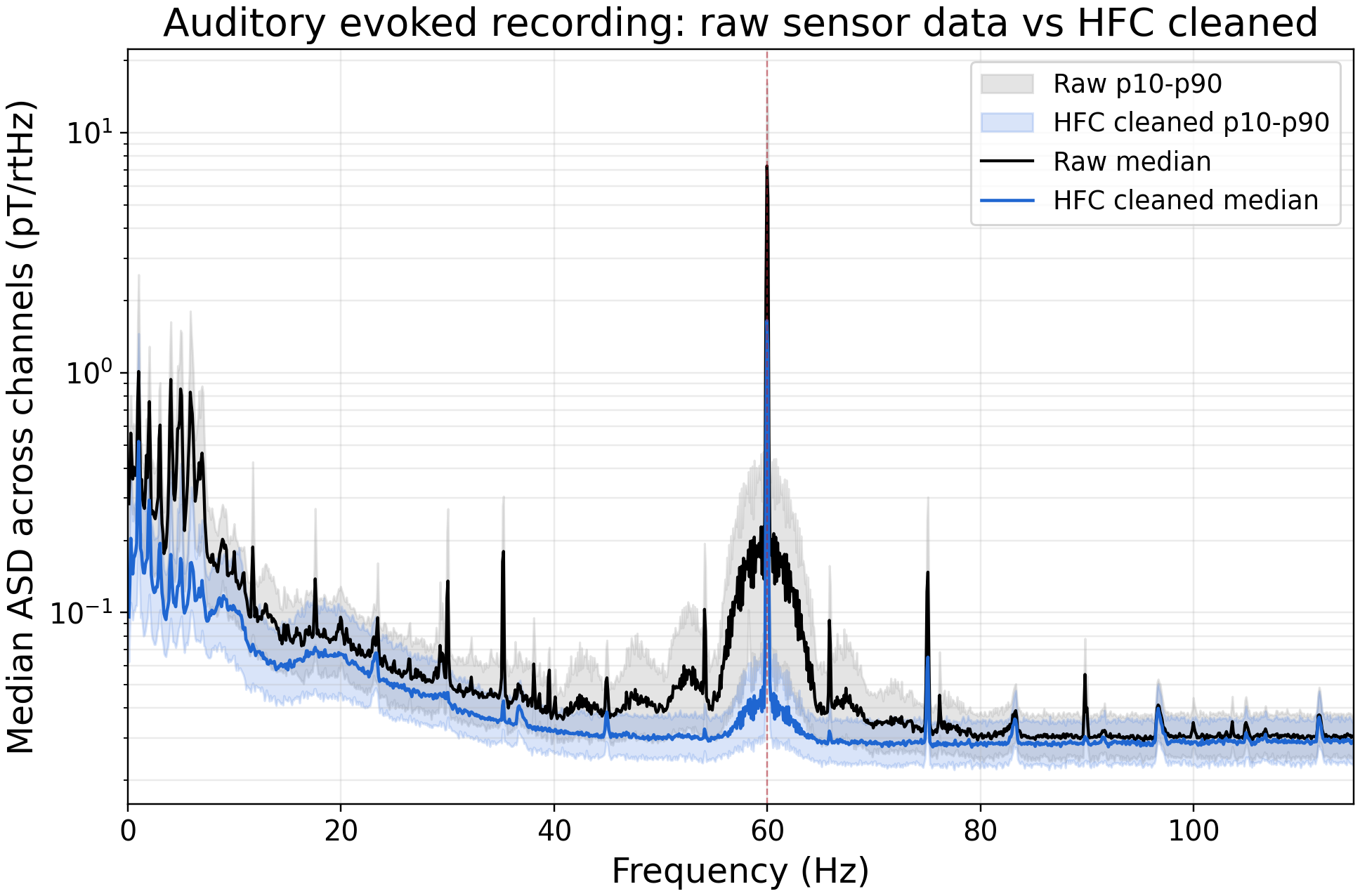
QuSpin provides first-order HFC correction via quspin.exe hfc, and that is what the example below demonstrates. HFC removes the best-fitting spatially uniform magnetic field from the array at each time sample, suppressing common-mode environmental noise while preserving channel-level signal. Flat or geometry-invalid channels are automatically excluded from the fit. Figure 9 shows the raw vs. HFC amplitude spectral density before and after correction.
Example Python Script
The two-step script below converts your recording to FIF with sensor geometry embedded, then applies HFC correction using the quspin.exe CLI.
import subprocess
from pathlib import Path

# ── Set your paths ────────────────────────────────────────────────
QUSPIN_EXE       = Path(r".\quspin.exe")
INPUT_LVM        = Path(r"C:\your_data\aer_recording.lvm")
LOCALIZATION_CSV = Path(r"C:\your_results\localization_results.csv")
CALIBRATED_FIF   = Path(r"C:\your_results\aer_calibrated.fif")
HFC_FIF          = Path(r"C:\your_results\aer_hfc.fif")
# ─────────────────────────────────────────────────────────────────

# Step 1 — Convert to FIF and embed sensor geometry
subprocess.run([
    str(QUSPIN_EXE), "fiff",
    "-i", str(INPUT_LVM),
    "-o", str(CALIBRATED_FIF),
    "-l", str(LOCALIZATION_CSV),
    "--apply-pos-orients",
    "--apply-cals",
    "--verbose",
], check=True)

# Step 2 — Apply HFC
subprocess.run([
    str(QUSPIN_EXE), "hfc",
    "--input-path", str(CALIBRATED_FIF),
    "--output-path", str(HFC_FIF),
    "--verbose",
], check=True)

print(f"HFC-corrected FIF saved to: {HFC_FIF}")
LCMV Beamforming
The script run_landmark_guided_lcmv_beamformer.py performs source localization on the HFC-corrected FIF using a landmark-guided vector LCMV beamformer, identifying bilateral auditory sources in the temporal region without requiring an MRI or conductor model. All beamformer computation is done in SCF; source coordinates are converted to HCF only for reporting and visualization. The script is thoroughly commented and closely follows the MNE-Python tutorials for epoching, covariance estimation, and beamforming concepts. The pipeline runs in five stages:
Pipeline overview
- Load the FIF, identify usable channels, apply HFC and bandpass filtering, extract trigger-locked epochs, compute the evoked average.
- Estimate baseline and active covariance matrices; compute the regularized inverse.
- Use HALO Pen landmarks to build a bilateral temporal candidate source grid in SCF.
- Run a vector LCMV beamformer at every candidate; score each by active-to-baseline power ratio.
- Select the top source per hemisphere; project its spatial filter onto all epochs to produce virtual-electrode time courses.
Epoching and Evoked Average
The script opens the calibrated FIF with mne.io.read_raw_fif and builds a per-channel model that flags channels as usable only if they have valid HALO-localized positions, finite sensitivity-axis vectors, and non-flat signals. A first-order HFC projection is then applied in software — identical in effect to quspin.exe hfc — and the data are bandpass-filtered from 3–45 Hz using a zero-phase 4th-order Butterworth filter.
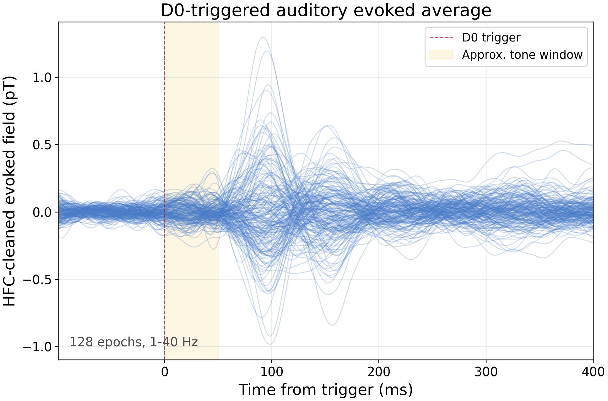
Trigger events on the D0 channel are detected with mne.find_events. Epochs of −100 to +400 ms are cut around each event and baseline-corrected by subtracting the mean of the pre-stimulus window (−100 to 0 ms). Epochs that would extend beyond the recording boundary are discarded. The sensor-level evoked average across all valid trials is shown in Figure 10; the auditory M100 response is clearly visible near 100 ms post-stimulus across the OPM channel array.
Covariance Estimation
Two covariance matrices are estimated from the epoched data: a baseline matrix from the pre-stimulus window (−100 to 0 ms) and an active matrix from the expected response window (50–180 ms). Pooling samples across all trials gives stable estimates even with a modest number of epochs. The baseline matrix serves double duty: it is used to compute the regularized filter inverse, and as the noise reference against which active source power is normalized.
Regularization uses diagonal loading — adding a scaled identity matrix equal to 1% of the mean sensor variance before inverting — which prevents numerical blow-up when the covariance matrix is ill-conditioned. See the MNE tutorials on covariance estimation for guidance on choosing regularization and estimation strategies appropriate to your dataset.
Landmark-Guided Search Grid
Instead of scanning the whole head, the search is constrained to the bilateral temporal region. HALO Pen touch clusters at the nasion, below the nose, and at each ear (3 touches each, averaged) define a right-handed anatomical coordinate basis using Gram-Schmidt orthogonalization — yielding lateral, anterior, and superior unit vectors in SCF. A dense candidate grid is then sampled at 5 mm steps from each ear landmark: 20–65 mm medially, ±25 mm anterior/posterior, and 20–70 mm superiorly. All candidate positions are expressed in SCF to match the sensor geometry.
Vector LCMV Source Scan
At each candidate location a free-space magnetic dipole leadfield is computed in SCF from the HALO-localized sensor positions and sensitivity axes — no MRI or conductor model is required. The 3 × Nsensors LCMV weight matrix is derived from the regularized covariance inverse. The optimal source orientation is found by solving the generalized eigenvalue problem between the active and baseline source covariance matrices: the eigenvector corresponding to the largest eigenvalue gives the axis that maximizes the active-to-baseline power ratio. This ratio is used as the scan score.
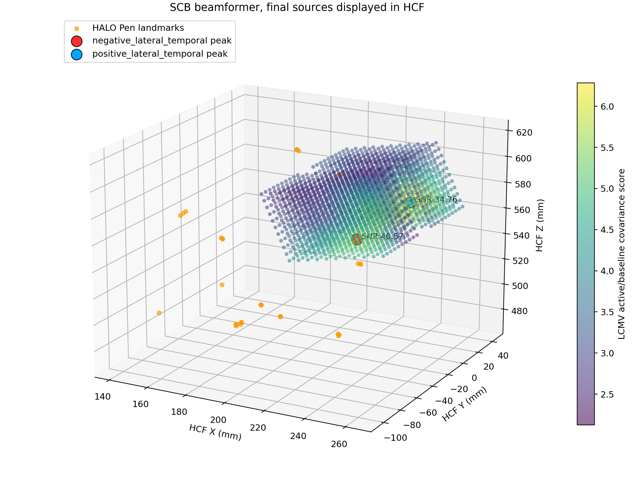
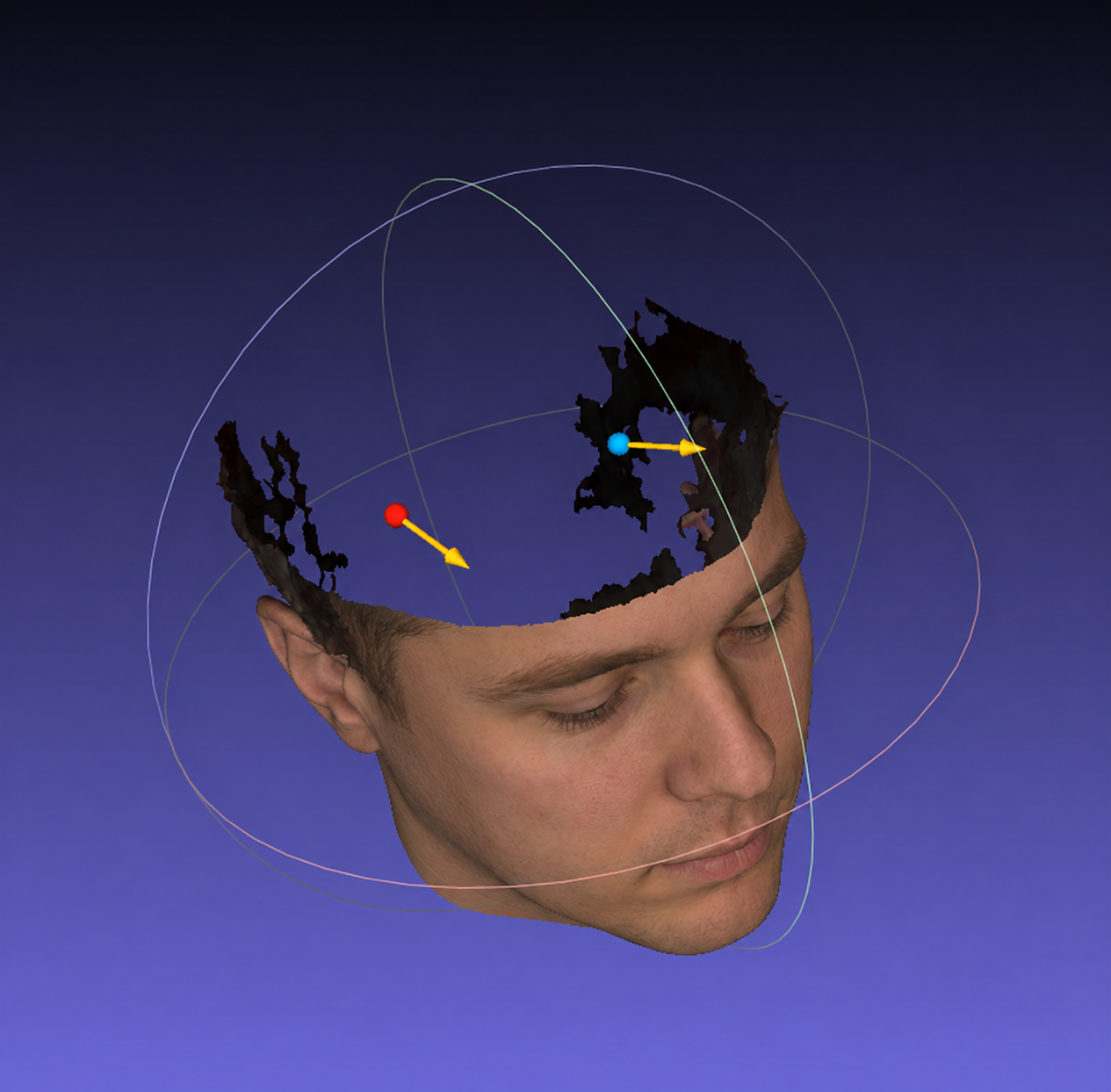
Figure 11 shows the full scan landscape — every candidate location colored by its score — with the selected bilateral peaks marked. Figure 12 shows those peaks overlaid on the subject 3D scan in HCF.
Virtual Electrodes and Source Waveforms
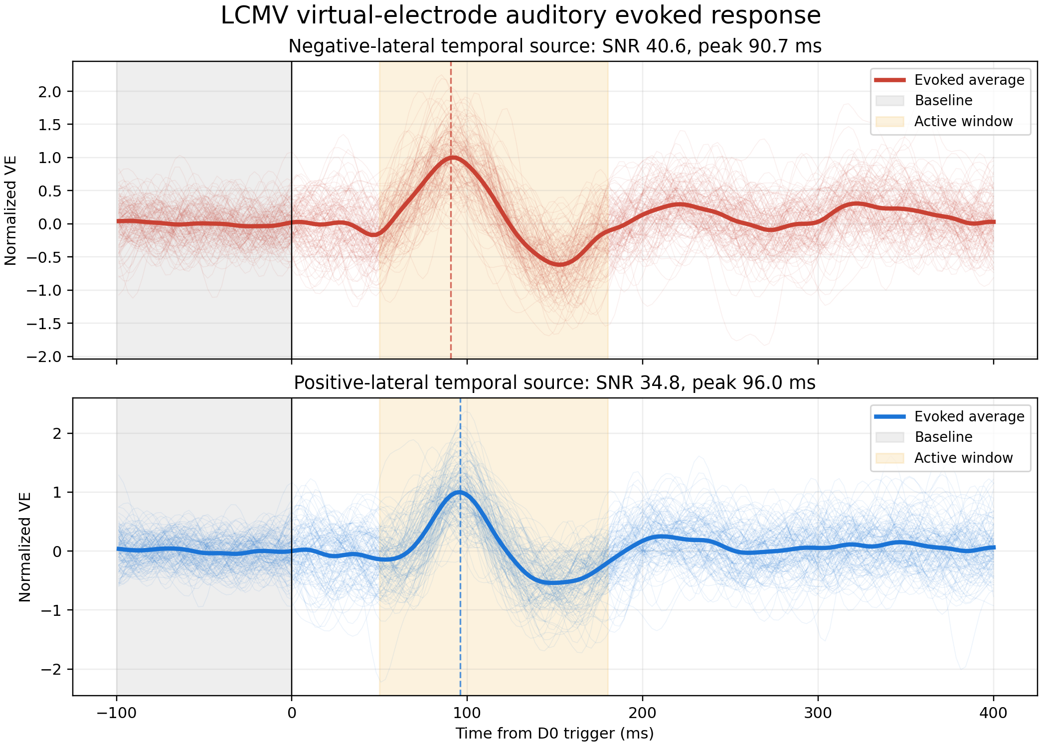
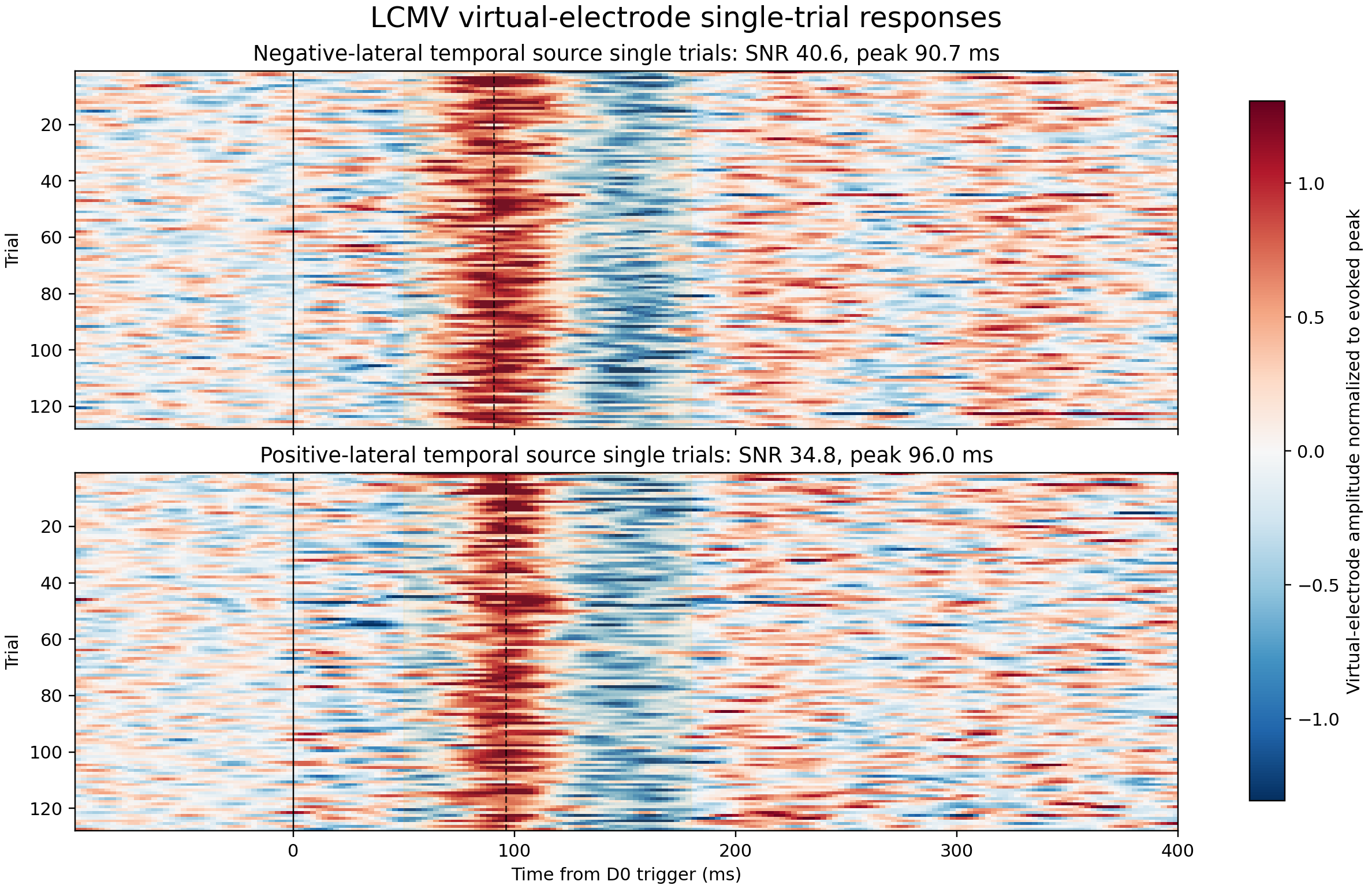
The highest-scoring candidate per hemisphere is selected. Its scalar LCMV spatial filter — the 3D beamformer weights projected onto the optimal source orientation — is applied to every individual epoch, converting the multichannel sensor array into a single virtual-electrode time course per source. The sign is normalized so the evoked peak is positive (dipole polarity is inherently sign-ambiguous). Figure 13 shows the evoked average overlaid on individual trials for each hemisphere; Figure 14 shows the corresponding single-trial heatmaps, which reveal the trial-by-trial consistency of the auditory response at source level.
Example Python Script
Download run_landmark_guided_lcmv_beamformer.py, open it in a text editor, and fill in the USER CONFIGURATION block at the top of the file with your own paths, FrameAlign transform, and parameters. Then run: python run_landmark_guided_lcmv_beamformer.py
# ═══════════════════════════════════════════════════════════════════════════════
# USER CONFIGURATION — edit these values before running
# ═══════════════════════════════════════════════════════════════════════════════

# ── File paths ─────────────────────────────────────────────────────────────
INPUT_FIF = Path(r"C:\your_data\aer_calibrated.fif")
# Calibrated FIF produced by quspin.exe fiff (sensor positions and gains embedded).

PEN_POINTS_CSV = Path(r"C:\your_data\halo_pen_tip_points_xyz.csv")
# HALO Pen tip point CSV produced by quspin.exe fiducial (columns X, Y, Z in SCB metres).

RESULTS_DIR = Path(r"C:\your_results\beamforming")
# All output files (CSVs, PNGs, OBJ meshes, summary JSON) are written here.

# ── SCF-to-HCF transform (from FrameAlign) ─────────────────────────────────
# Replace with the 4×4 similarity transform exported from your FrameAlign session.
# Row-major: p_hcf_mm = SCB_TO_HCF @ [x_scb_m, y_scb_m, z_scb_m, 1]^T
SCB_TO_HCF = np.array(
    [
        [XX.X, XX.X, XX.X, XX.X],
        [XX.X, XX.X, XX.X, XX.X],
        [XX.X, XX.X, XX.X, XX.X],
        [0.0,  0.0,  0.0,  1.0],
    ],
    dtype=float,
)

# ── Stimulus trigger ────────────────────────────────────────────────────────
TRIGGER_CHANNEL = "D0"          # Trigger channel name in the FIF file

# ── Epoch timing (seconds, relative to trigger onset) ──────────────────────
EPOCH_TMIN_SEC      = -0.10     # Pre-stimulus start
EPOCH_TMAX_SEC      =  0.40     # Post-stimulus end
BASELINE_WINDOW_SEC = (-0.10, 0.0)   # Baseline correction window
ACTIVE_WINDOW_SEC   = ( 0.05, 0.18)  # Expected response window for scoring

# ── Bandpass filter ─────────────────────────────────────────────────────────
FILTER_HZ = (3.0, 45.0)         # (low_hz, high_hz) — 4th-order Butterworth

# ── Covariance regularization ───────────────────────────────────────────────
COV_REG = 0.01                  # Diagonal loading: 0.01 = 1 % of mean sensor variance

# ── HALO Pen landmark point indices (1-based row numbers in PEN_POINTS_CSV) ─
# Each landmark should be touched 3 times in sequence.
# Update these if you touched landmarks in a different order or count.
NASION_INDICES         = [4, 5, 6]
NOSE_INDICES           = [16, 17, 18]
RIGHT_EAR_INDICES      = [30, 31, 32]
LEFT_EAR_PROXY_INDICES = [27, 28, 29]

# ── Bilateral temporal candidate search grid (metres from each ear) ─────────
MEDIAL_OFFSETS_M    = np.arange(0.020, 0.066, 0.005)   # 20–65 mm medial, 5 mm step
POSTERIOR_OFFSETS_M = np.arange(-0.025, 0.026, 0.005)  # ±25 mm anterior/posterior
SUPERIOR_OFFSETS_M  = np.arange(0.020, 0.071, 0.005)   # 20–70 mm superior

# ── Plot display limit ──────────────────────────────────────────────────────
TRIAL_PLOT_MAX_TRACES = 128     # Max individual trial traces shown in VE plot

# ═══════════════════════════════════════════════════════════════════════════════
# END USER CONFIGURATION
# ═══════════════════════════════════════════════════════════════════════════════
SNR note. These SNR values are measured on the averaged LCMV virtual electrode across 128 trials, with the source location and orientation selected from the active-versus-baseline contrast. The response is strong, but this should not be interpreted as single-trial SNR. For a publication-grade estimate, use split-half or held-out trials, bootstrap confidence intervals, and/or a null control.
Moment-arrow convention. The LCMV dipole orientation is an axis, not a uniquely signed arrow — flipping the moment and flipping the virtual-electrode sign gives an identical sensor prediction. For the OBJ visualization the two moment arrows are sign-normalized to point in a generally parallel direction. The source table retains the original LCMV orientation components.