
Gradiometer mode uses two synchronized magnetometers to reduce environmental magnetic noise. The reading from one sensor is subtracted from the other:
Gradiometer signal = Sensor A − Sensor B
This works best when both sensors measure approximately the same background noise, but the signal of interest is different at each sensor. Subtraction removes much of the shared — or common-mode — noise while preserving the local signal.
The distance between the two sensors is called the baseline. As a useful rule of thumb, the baseline should be roughly comparable to the distance between the sensors and the object being measured. Environmental noise sources should ideally be much farther away, so that their fields are nearly the same at both sensors.
For example, consider an unexploded ordnance (UXO) object approximately 1 metre from the sensors, with a 1‑metre sensor baseline. The UXO field may be noticeably different at each sensor, while distant geomagnetic and environmental noise is similar. Subtraction can therefore reduce the background while retaining the UXO signal.
If the same object is 10 metres away but the baseline remains 1 metre, both sensors will measure much more similar fields from the object. In that case, subtraction may reduce the desired signal along with the environmental noise, making a simple gradiometer less helpful.
In the example below, two scalar magnetometers were placed close together in a noisy laboratory. They detected nearly the same environmental noise, so subtraction removed most of it. Some residual gradient noise remained because computers and other magnetic equipment were located close to the sensors.
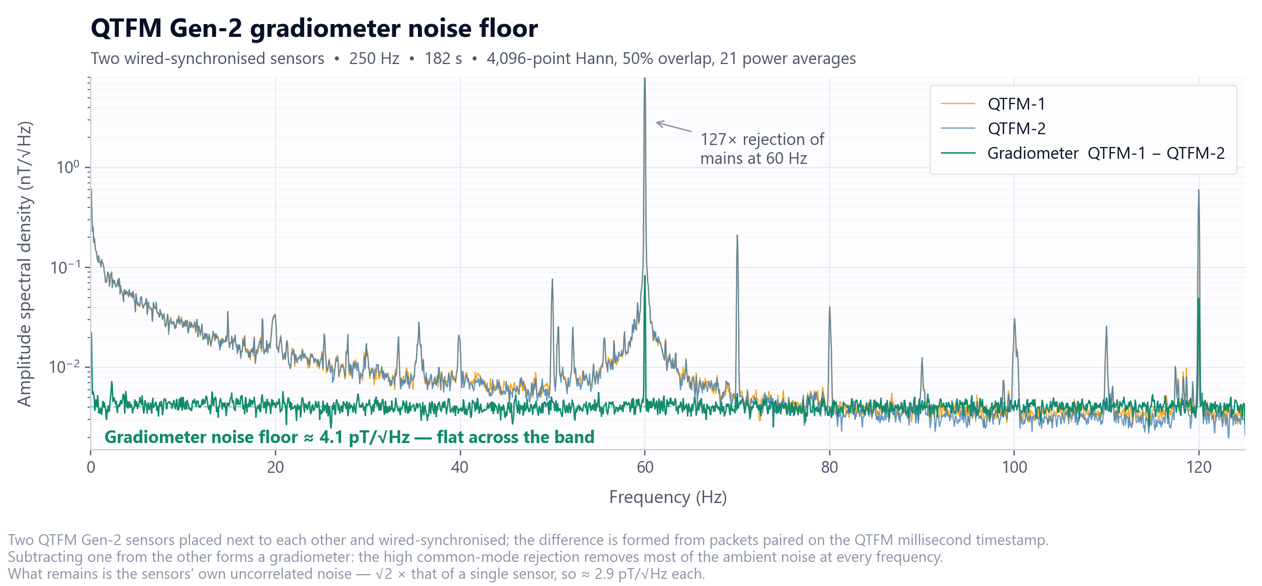
Once the common environmental field has cancelled, what is left is the two sensors’ own uncorrelated noise. Here the gradiometer noise is 4.1 pT/√Hz, which puts each sensor at roughly 4.1 ÷ √2 ≈ 2.9 pT/√Hz — so this measurement is limited by the sensors themselves, not by the room.
With a larger sensor array, advanced signal-processing methods such as independent component analysis (ICA) or beamforming can sometimes separate signals according to their spatial or temporal characteristics. These approaches require more sensors, careful calibration, and greater processing complexity, so they are rarely used in routine gradiometer measurements.
Resources
- Gradiometer software installer, supporting up to 8 sensors — QTFM_Simple_Gradiometer_Setup_1.4.1.exe (47 MB, Windows x64). Installs the application and adds it to the Start menu.
-
Portable copy with source code —
QTFM_Simple_Gradiometer_1.4.1_Windows_x64.zip
(63 MB). The ZIP includes the Windows application — the executable is in the
Appfolder — and the complete GPL open-source Python code for the plotting software in theSourcefolder. - Sensor setup and synchronization instructions — Syncing Your Gen‑2 QTFM Sensors. The gradiometer software uses wired Master/Slave sync through the Standard Comms Board (SCB).
- Sample gradiometer data — qtfm-gradiometer-sample-data.csv (4 MB). The 182 s two-sensor recording used in the figure above: millisecond timestamp, both sensor readings in nT, and their difference.
Previous software versions
| Version | Installer | Portable ZIP with source |
|---|---|---|
| 1.0.0 | QTFM_Simple_Gradiometer_Setup_1.0.0.exe (38 MB) | QTFM_Simple_Gradiometer_1.0.0_Windows_x64.zip (53 MB) |
Technical note Sensor A − Sensor B is a magnetic-field difference in nT. Dividing this difference by the sensor baseline provides an approximate magnetic gradient in nT/m. If both sensors have equal, uncorrelated noise, the noise of one sensor can be estimated by dividing the measured gradiometer noise by √2.